The size–luminosity relationship of quasar narrow-line regions

In some distant galaxies – many of them so distant that the light we see from them was emitted some 10 billion years ago – a supermassive black hole, containing the mass of millions or billions of Suns, is surrounded by a disk of gas. As this gas falls into the black hole, its energy is converted into radiation across the electromagnetic spectrum, forming an extraordinarily luminous object known as a quasar. Quasars are so luminous that they can outshine entire galaxies, and thus they are a force to be reckoned with in their own host galaxies. Astronomers studying galaxy formation are particularly interested in how they formation of a quasar can lead to feedback on the host galaxy, whereby the quasar is so powerful that it blows away gas in the galaxy and diminishes the formation of more stars.

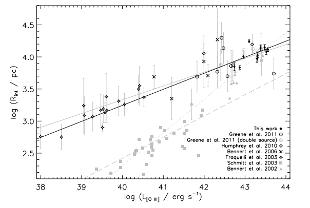
Needless to say, quasars are very complex objects. Their radiative power varies by many orders of magnitudes, and their host galaxies have all sorts of various properties. Any similarity across quasars is of great interest, since they are naturally so diverse. And indeed, there is a striking similarity which begged for an explanation. Type II quasars, in which the quasars themselves are obscured by dust and gas surrounding the black hole, have a “size” set by the amount of gas in the host galaxies which they illuminate. This size appears to be strongly correlated with their luminosities.

This paper aims to explain the relationship in terms of a simple model of quasar radiative feedback. There are two main facets to explain: first, why are size and luminosity related in the manner that they are? Second, why is the relationship so tight, given the wide variation in the quasar population?

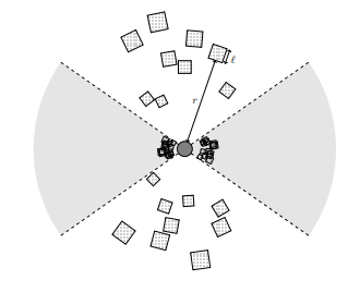
We can approach these questions by thinking about the physics within gas clouds surrounding the quasar. Shown below is a schematic view of the quasar, with a dense ring of clouds obscuring the quasar light, and illuminated clouds in the remaining bicone.

The temperature in these clouds is fixed by a balance between the rates of photoionization of atoms and their recombination to be about $10^4\,\text{K}$. Their pressure is fixed by balance with the radiation pressure, so we have

where $L$ is the quasar luminosity. By the ideal gas law, the number density of particles in the clouds is given by

If we know the cloud mass $m_c$, then the volume of clouds is given by

where $m_p$ is the proton mass, a good approximation to the average mass of particles. The only parameter we needed here to describe a cloud was its mass $m_c$. The only remaining parameter is how many clouds there are, which is set by their covering factor $\Omega$, the fraction of the sky above the quasar which is covered by clouds.

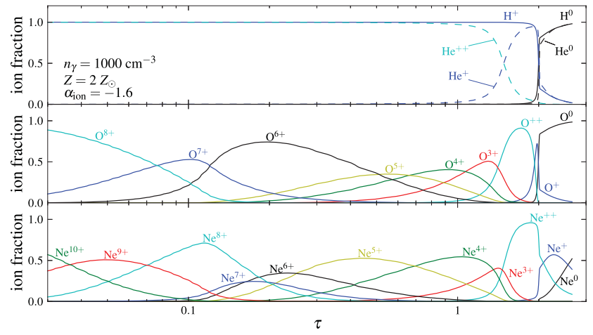
Then comes the tricky part: what happens when these clouds are impacted by radiation from the quasar? The short answer is photoionization: atoms are going to be stripped apart by the energy of the photons. This is simple enough for a hydrogen atom, its one electron is either bound or ionized. It’s more complicated for an atom like oxygen, which can be ionized between 0 and 8 times. We are especially interested in oxygen, because the size-luminosity relationship shown above uses a size metric based on the luminosity of an emission line coming from doubly ionized oxygen, called [O III].

Luckily, Stern et al. (2014) already computed the ionization structure of oxygen in clouds illuminated by quasars. The clouds end up forming a layered structure. The layer closest to the quasar feels the full brunt of its radiation, and oxygen in this layer will be fully ionized. Successive layers are hit with less and less radiation power, and so oxygen is less and less ionized.

Using the Stern et al. results, we can tally up how much [O III] light is coming from each of the clouds. Summming this all up gives the [O III] luminosity, which is the horizontal axis of the size-luminosity plot above. If we tally it up more carefully, we can predict what a telescope would see by measuring the [O III] light pixed by pixel across the galaxy. In particular, we can find the distance from the center of the galaxy at which the [O III] surface brightness falls below a certain cutoff, which defines the size used on the vertical axis of the same plot.

So, all told, we only need to fix the cloud mass $m_c$ and the cloud covering factor $\Omega$. Once we have that, we can compute the [O III] size and luminosity as a function of the total quasar luminosity $L$, and compare the size-luminosity relationship with the observed one. Is the relationship similar? Is it relatively tight, i.e., not strongly dependent on $m_c$ or $\Omega$?

Yes, and yes. Below is a plot from our paper showing the predicted size luminosity relationship with parameters in the range $m_c = 10^5$ – $10^7\,M_\odot$ and $\Omega = 3\times 10^{-4}$ – $3\times 10^{-2}$; two orders of magnitude spanned in each parameter. At high luminosities, the predictions agree quantitatively with Liu et al. (2013), the data in the plot above. At low luminosities there is some disagreement, but our predictions agree much better with some newer observations (Fischer et al. 2018). In addition, there is good agreement between our model and MaNGA data.

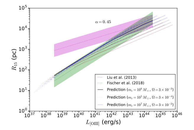
In addition to the good agreement with the data, the model seems to go a long way towards explaining the tightness of the fit. Even varying both parameters by two decades produces relatively little spread in the predictions. In hindsight this can be explained rather succinctly. If we increase $\Omega$, e.g. by adding ten times as many clouds to the galaxy, then we expect to see ten times as much [O III] light. The size will also increase by some amount, which depends on the slope of the [O III] surface brightness profile. Now, what would happen if instead of adding ten times more clouds, we made the quasar ten times brighter? Then again we would see ten times more [O III] light, and the size would increase by some amount – as it turns out, the very same amount as if we increased the number of clouds. So changing $\Omega$ is equivalent to changing $L$, which means we stay on the same curve.

Now what if we increase the mass $m_c$? Well, all the [O III] light is coming from a particular layer of the clouds. So if we add more mass, we’re essentially piling more gas onto the back of the cloud, where [O III] emission isn’t happening. So, again, no change in the [O III] size/luminosity relationship.

This line of argument seems to suggest that there should be exactly zero spread in the relationship, but we do see some. The reason is that not all of the clouds are thick enough to exhibit any [O III] emission at all. These thin clouds are called “matter-bounded,” as opposed to “ionization-bounded”: their [O III] emission is bounded not by the amount they are irradiated, but by how massive they are. So when we increase $m_c$, some of these clouds become massive enough to emit [O III], which changes the size/luminosity relationship.

Given that this model seems to reproduce the [O III] size and luminosity fairly well, could we use it to address other properties of these quasars and their host galaxies? One relatively simple and interesting quantity is the total mass contained in these clouds. Previous methods for estimating the mass are based on the total luminosity coming from hydrogen emission lines. Hydrogen lines only come from one layer of the clouds, and so these methods can miss a lot of mass. We can use our model to compute a total cloud mass, and we end up with a value roughly 10 times greater than the hydrogen-based estimates.

There’s much, much more to be said and asked about radiative feedback of quasars. One follow-up study is here. One overarching question is how exactly do quasars regulate galaxy formation? This is a key question in understanding how $\Lambda$-CDM, the prevailing model of cosmology, explains the present distribution of matter into galaxies in our universe.