Catalan Numbers in Perturbation Theory
Remarks on the perturbation theory for problems of Mathieu type (Arnol'd)
 Download the notebook
Catalan numbers are everywhere. Quite famously, in volume 2 of his Enumerative Combinatorics, Richard P. Stanley gives 66 different interpretations of these numbers. They are given by
\[C_n = \frac{1}{n+1}\binom{2n}{n},\]and the first few are $1, 1, 2, 5, 14, 42, \ldots$. They are sequence A000108 in the Online Encyclopedia of Integer Sequences, and that very low call number might be another indication of their importance.
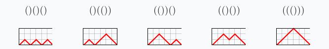
To give just one of the $\ge 66$ interpretations of these numbers, consider the problem of balanced parentheses. We would like to know, given $n$ pairs of parentheses, how many ways they can be arranged to give a balanced expression. When $n = 1$, there is only one way, $()$. For $n = 2$, we have two choices, $()()$ and $(())$. For $n = 3$, five choices:
\[((())), (())(), ()(()), (()()), ()()()\]And for $n = 4$, there are fourteen choices:
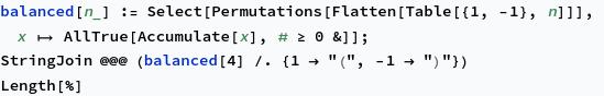


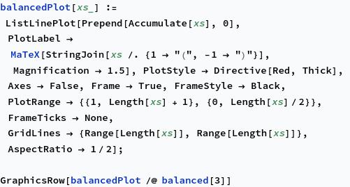
Note the approach we took in this last case: we think of “(“ as +1 and “)” as -1, and then make sure that as we read through the expression, we never dip below 0, that is, we never close a parenthesis before it is opened. This is precisely what it means to have a balanced expression. We can use this idea to give a graphical interpretation to balanced parentheses, by plotting the partial sums that are used in the code snippet above. Here are those plots for $n = 3$:
Let’s prove that these counts are given by the Catalan numbers. Let $a_n$ be the number of balanced expressions of $n$ pairs of parentheses. To write down a balaned expression, we always start by writing down a left parenthesis. Eventually that left parenthesis has to be closed, and then we can add more parentheses afterwards. So a balanced expression of $n$ pairs has the following form:

This leads to the recursion
\[a_n = \sum_{m=0}^{n-1} a_m a_{n-m-1},\qquad a_0 = 1.\]To solve the recursion, we can use a generating function. Let
\[f(x) = \sum_{n=0}^\infty a_n x^n.\]Then, formally,
\[f^2 = \sum_{n=0}^\infty \left(\sum_{m=0}^n a_m a_{n-m}\right) x^n.\]Comparing with the recursion relation above, we have
\[f = 1 + xf^2,\]and solving this gives
\[f = \frac{1 - \sqrt{1 - 4x}}{2x}.\]We can check quickly that we have the correct generating function:
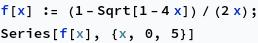

Better yet, we can use the generating function to find an explicit form for $a_n$. We have
\[\sqrt{1-4x} = (1-4x)^{1/2} = \sum_{n=0}^\infty (-4)^n \binom{1/2}{n} x^n = 1 - \sum_{n=1}^\infty \frac{2}{n}\binom{2n-2}{n-1} x^n.\]This gives
\[f = \sum_{n=0}^\infty \frac{1}{n+1}\binom{2n}{n} x^n,\]so indeed $a_n = C_n$.
The Catalan numbers appear in a somewhat surprising way in the context of eigenvalue perturbation theory. Michael Scheer and I noticed this and had lots of fun working it out. We eventually realized that this result appears in an old paper of V. I. Arnol’d, cited above. Instead of borrowing Arnol’d’s succinct discussion, though, I’ll outline how Michael and I came to the same ideas. This should give an idea of how a mere mortal (i.e., not Arnol’d) could notice these patterns, and it also comes with a useful visual mnemonic for the terms in eigenvalue perturbation theory.
Perturbation Theory
As any quantum mechanic knows, determining the dynamics of a quantum system boils down to solving an eigenvalue problem of the form
\[H\ket{\psi_n} = E_n\ket{\psi_n},\]
where $H$ is the Hamiltonian operator for the system and $E_n$ is an energy eigenvalue. The time evolution of the eigenstates is then given by
\[\ket{\psi_n(t)} = e^{-iE_n t/\hbar}\ket{\psi_n(0)},\]and so by decomposing the initial state into the energy eigenstates and using this result, we can find the time evolution of any initial state.
Cool. So we need to solve eigenvalue problems. Unfortunately, this is quite hard in general. For a finite-dimensional system, we at least have the option of calculating all the matrix elements $H_{ij} = \braket{\phi_i|H|\phi_j}$ and computing the eigenvalues numerically. For an infinite-dimensional system, we can’t even fall back on this brute force approach; we need some more clever way of getting at the spectrum of the Hamiltonian.
A common approach is perturbation theory. If the Hamiltonian can be expressed as a small correction to a Hamiltonian whose spectrum we know, then the new spectrum should be a small correction to the old spectrum. Let’s see how this works out.
We write $H = H_0 + \epsilon V$, and assume we know the eigenvalues $E_n^{(0)}$ and normalized eigenvectors $\ket{n^{(0)}}$ of $H_0$:
\[H_0 \ket{n^{(0)}} = E_n^{(0)} \ket{n^{(0)}}.\]We also assume all the $E_n^{(0)}$ are distinct. Then, let $E_n$ and $\ket{n}$ be the eigendata of $H$:
\[H\ket{n} = E_n \ket{n}.\]We can write these as series in $\epsilon$:
\[E_n = E_n^{(0)} + \epsilon E_n^{(1)} + \ldots, \qquad \ket{n} = \ket{n^{(0)}} + \epsilon \ket{n^{(1)}} + \ldots.\]Substituting this into the eigenvalue equation and using $H = H_0 + \epsilon V$, we find
\[E_n^{(0)}\ket{n^{(0)}} + \epsilon V \ket{n^{(0)}} + \epsilon H_0 \ket{n^{(1)}} + \mathcal{O}\left(\epsilon^2\right) = E_n^{(0)}\ket{n^{(0)}} + \epsilon E_n^{(1)}\ket{n^{(0)}} + \epsilon E_n^{(0)}\ket{n^{(1)}} + \mathcal{O}\left(\epsilon^2\right).\]Canceling the first terms and acting with $\bra{n^{(0)}}$, we find at order $\epsilon$ that
\[\braket{n^{(0)}|V|n^{(0)}} + \braket{n^{(0)}|H_0|n^{(1)}} = \braket{n^{(0)}|E_n^{(1)}|n^{(0)}} + \braket{n^{(0)}|E_n^{(0)}|n^{(1)}}.\]The second terms cancel because $\bra{n^{(0)}}H_0 = \bra{n^{(0)}}E_n^{(0)}$, and so we find
\[E_n^{(1)} = \braket{n^{(0)}|V|n^{(0)}}.\]We can then insert this back into the equation above, giving
\[V \ket{n^{(0)}} + H_0 \ket{n^{(1)}} = \braket{n^{(0)}|V|n^{(0)}}\ket{n^{(0)}} + E_n^{(0)}\ket{n^{(1)}}.\]Acting with $\bra{m^{(0)}}$, we find
\[\braket{m^{(0)}|V|n^{(0)}} = (E_n^{(0)}-E_m^{(0)})\braket{m^{(0)}|n^{(1)}}.\]Normalization of $\ket{n}$ requires $\braket{n^{(0)}|n^{(1)}} = 0$, and we can solve for all the other components of $\ket{n^{(1)}}$ from the above, so we find
\[\ket{n^{(1)}} = \sum_{m\neq n} \frac{\braket{m^{(0)}|V|n^{(0)}}}{E_n^{(0)}-E_m^{(0)}}\ket{m^{(0)}}.\]To find the higher-order corrections, the typical approach followed in textbooks is to just keep on chugging: look at the $\epsilon^n$ terms in the eigenvalue equation, substitute what we found for the $(n-1)$th order terms, and solve for the $n$th order terms. This is a massive pain. Life gets much easier when we realize that $E_n^{(1)}$ and $\ket{n^{(1)}}$ are just the derivatives of $E_n$ and $\ket{n}$ with respect to $\epsilon$, evaluated at $\epsilon = 0$. We can use these derivatives to find any higher terms. For example,
\[E_n^{(2)} = \frac{1}{2}\left.\d{E_n^{(1)}}{\epsilon}\right|_{\epsilon = 0} = \frac{1}{2}\left(\frac{d}{d\epsilon}\braket{n|V|n}\right)_{\epsilon = 0}\]Using our expression above to differentiate $\ket{n}$, we find
\[E_n^{(2)} = \sum_{m\neq n} \frac{\braket{n^{(0)}|V|m^{(0)}}\braket{m^{(0)}|V|n^{(0)}}}{E_n^{(0)}-E_m^{(0)}}.\]What if we want $E_n^{(3)}$? Then we take another derivative, which requires using our rules to differentiate every state and every energy appearing above. This quickly gets messy, but it can be done. Later we’ll show some tricks to make this process much easier.
(An)harmonic Oscillator
As an example of applying perturbation theory, consider the Hamiltonian of a harmonic oscillator,
\[H_0 = \frac{p^2}{2m} + \frac{1}{2}m\omega^2 x^2.\]It is well-known that if we write
\[x = \sqrt{\frac{\hbar}{2m\omega}}\left(a^\dagger + a\right), \qquad p = i\sqrt{\frac{\hbar m\omega}{2}}\left(a^\dagger - a\right)\]then we find
\[H = \hbar\omega\left(a^\dagger a + \frac{1}{2}\right).\]We then define the vacuum by $a\ket{0} = 0$, and the normalized energy eigenstates are given by
\[\ket{n} = \frac{1}{\sqrt{n!}} \left(a^\dagger\right)^n\ket{0}\]with $H_0 \ket{n} = \hbar\omega\left(n+\frac{1}{2}\right)\ket{n}$.
This solves the quantum harmonic oscillator problem. What if we then want to add an anharmonic term, such as $H = H_0 + \epsilon x^k$? To do perturbation theory, we first need to compute the matrix elements of $V = x^k$ in the basis of energy eigenstates. The easiest way to do this is to rewrite $x$ in terms of the ladder operators, and use the fact (which can be shown from the definitions and canonical commutation relations) that $\left\lbrack a, a^\dagger\right\rbrack = 1$. For instance:
\[\braket{2|\left(a^\dagger + a\right)^2|2} = \braket{2|\left(a^\dagger a + a a^\dagger\right)|2} = \frac{1}{2}\braket{0|a^2\left(a^\dagger a + a a^\dagger\right)\left(a^\dagger\right)^2|0} = \frac{1}{2}\braket{0|a^2\left(-1 + 2a a^\dagger\right)\left(a^\dagger\right)^2|0} = 5,\]where in the last step we use the normalization of $\ket{2}$ and $\ket{3}$. In general, it’s easy to show that the expectation value of this operator for $\ket{n}$ is $2n+1$.
We can easily automate this process, by telling Mathematica how to move annihilation operators to the right (a process called normal-ordering):
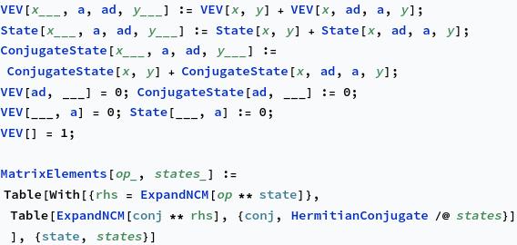
Note that there’s lots of other behind-the-scenes code here, download the notebook to see it all. Now let’s make ourselves a basis of the first few eigenstates and get the matrix elements of $x^2 \propto \left(a^\dagger + a\right)^2$:
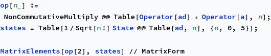
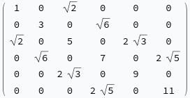
As expected, we see the values $2n+1$ along the diagonal. We also find
\[\braket{n+2|\left(a^\dagger + a\right)^2|n} = \sqrt{(n+2)(n+1)},\]which is simple to prove.
We don’t have to use perturbation theory to add an $x^2$ potential, because in this case we still have a harmonic oscillator. With an extra $V = \frac{\epsilon}{2}m\omega^2 x^2$, we effectively change $\omega \mapsto \omega\sqrt{1+\epsilon}$, and so the energy levels become
\[E_n = \hbar\omega\sqrt{1+\epsilon}\left(n + \frac{1}{2}\right) = E_n^{(0)}\left(1 + \frac{1}{2}\epsilon - \frac{1}{8}\epsilon^2 + \ldots\right).\]Since we know this, though, we can check that perturbation theory gives us the right answer. We have
\[V = \frac{1}{2}m\omega^2 x^2 = \frac{1}{4}\hbar\omega \left(a^\dagger + a\right)^2.\]Thus,
\[E_n^{(1)} = \frac{1}{2}\hbar\omega\left(n+\frac{1}{2}\right),\]as expected. Better yet,
\[E_n^{(2)} = \frac{\braket{n|V|n+2}\braket{n+2|V|n}}{E_n-E_{n+2}} + \frac{\braket{n|V|n-2}\braket{n-2|V|n}}{E_n-E_{n-2}} = \frac{(\hbar\omega)^2}{16}\left(\frac{(n+2)(n+1)}{-2\hbar\omega} + \frac{n(n-1)}{2\hbar\omega}\right) = -\frac{1}{8}\hbar\omega\left(n+\frac{1}{2}\right).\]So indeed, perturbation theory is giving us the term by term expansion of the exact energy eigenvalues for the adjusted Hamiltonian.
Fun with Diagrams
To get our inspiration for dealing with perturbation theory at all orders, we need to compute $E_n^{(3)}$. Recall that this means differentiating
\[E_n^{(2)} = \sum_{m\neq n} \frac{\braket{n|V|m}\braket{m|V|n}}{E_n-E_m}.\]Let’s start with the eigenstates. When we hit the $\ket{n}$ or the $\bra{n}$, we get an additional sum over states which are not $n$:
\[\sum_{m\neq n} \sum_{k\neq n}\frac{\braket{n|V|m}\braket{m|V|k}\braket{k|V|n}}{(E_n-E_m)(E_n-E_k)} + \sum_{m\neq n} \sum_{k\neq n}\frac{\braket{n|V|k}\braket{k|V|m}\braket{m|V|n}}{(E_n-E_m)(E_n-E_k)} = 2\sum_{m\neq n} \sum_{k\neq n}\frac{\braket{n|V|m}\braket{m|V|k}\braket{k|V|n}}{(E_n-E_m)(E_n-E_k)}.\]When we hit the $\ket{m}$ or $\bra{m}$, the sum ranges instead over states which are not $m$:
\[\sum_{m\neq n} \sum_{k\neq m}\frac{\braket{n|V|m}\braket{m|V|k}\braket{k|V|n}}{(E_n-E_m)(E_m-E_k)} + \sum_{m\neq n} \sum_{k\neq m}\frac{\braket{n|V|k}\braket{k|V|m}\braket{m|V|n}}{(E_n-E_m)(E_m-E_k)}.\]If we swap the indices $m$ and $k$ in the second sum, the numerators become identical, and combining the denominators we end up with
\[\frac{\braket{n|V|m}\braket{m|V|k}\braket{k|V|n}}{E_m-E_k}\left(\frac{1}{E_n-E_m}-\frac{1}{E_n-E_k}\right) = \frac{\braket{n|V|m}\braket{m|V|k}\braket{k|V|n}}{(E_n-E_m)(E_n-E_k)}.\]Of course, this algebra only works for $k\neq n$, so we should remove those terms from both sums. In total, then, the terms from differentiating $\ket{m}$ and $\bra{m}$ are
\[\sum_{m\neq n}\sum_{k\neq n, m} \frac{\braket{n|V|m}\braket{m|V|k}\braket{k|V|n}}{(E_n-E_m)(E_n-E_k)} - 2\sum_{m\neq n}\frac{\braket{n|V|n}\braket{n|V|m}\braket{m|V|n}}{(E_n-E_m)^2}.\]We then almost have another copy of the double sum above; the only problem is that we’re missing the terms with $k = m$. But very conveniently, the precise terms we need to compensate are generated when we differentiate the denominator:
\[\sum_{m\neq n} \frac{\braket{n|V|m}\braket{m|V|n}(\braket{m|V|m}-\braket{n|V|n})}{(E_n-E_m)^2}.\]The other term combines nicely with what we just had to subtract off. Gathering all this up, we have in total
\[E_n^{(3)} = \frac{1}{3}\d{E_n^{(2)}}{\epsilon} = \sum_{m\neq n}\sum_{k\neq n} \frac{\braket{n|V|m}\braket{m|V|k}\braket{k|V|n}}{(E_n-E_m)(E_n-E_k)} - \sum_{m\neq n}\frac{\braket{n|V|n}\braket{n|V|m}\braket{m|V|n}}{(E_n-E_m)^2}.\]Somewhat miraculously, the terms have arranged themselves into a particular form: in the numerators, we have a cyclic arrangement of matrix elements of $V$. In the denominator, we have a product of differences between $E_n$ and other energy levels. And all of these other energy levels are simply summed over states not equal to $n$.
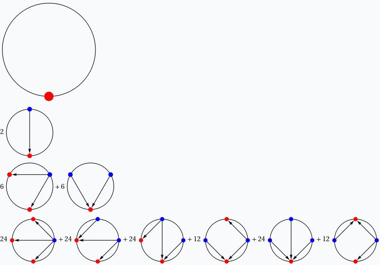
The appearance of these cyclic products of matrix elements makes it very tempting to draw some circles. As a first draft, we’ll do it like this: arrange $k$ points on a circle, and then draw $k-1$ directed edges between them, such that no point has both an incoming and an outgoing edge. We interpret every point with outgoing edges, the “sources”, as copies of $\ket{n}$; every point with incoming edges is a sum over $m_i\neq n$. The edges are energy differences in the denominator. Finally, for convenience, we add an overall factor of -1 if there is an even number of sources. In this notation, the first three energy corrections are

It turns out that all terms in perturbation theory, to all orders, can be written in terms of diagrams of this form. Proving this is an exercise in careful bookkeeping, taking derivatives of arbitrary diagrams and playing games like those above to resum into new diagrams. The end result is the following two rules for differentiating sources and sinks diagrammatically:

Now for the fun part: we can automate these rules and look at as many orders of perturbation theory as we’d like. We represent a diagram by a ChordGraph containing, for each point on the circle, a list of indices of the points to which it is connected by an edge (for sources) or an empty list (for sinks).
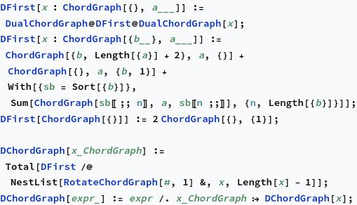
The DualChordGraph function (not shown) swaps the direction of all edges; to differentiate a sink, we differentiate the corresponding source in the dual graph and then take another dual.
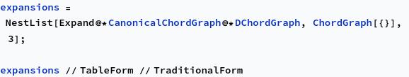
Now we can repeatedly differentiate the first correction and see what diagrams we get:
Note the extra factors of $n!$, because these are derivatives and not Taylor coefficients.
In the last row, we see something new happening: two of the diagrams come with factors of 12 instead of 24. But it turns out that these two diagrams give exactly the same sum. We can see this by moving one of the arrows to a different source (changing nothing, because the sources all represent $\ket{n}$), and then rotating the diagram.
This points to the fact that, although the arrow diagrams are pretty and form a very useful mnemonic for the first few corrections to the energy eigenvalues, they’re ultimately not a good representation of the terms because the origin point of arrows is not meaningful. All that really matters is the number of incoming arrows at each sink, so all we should keep track of is these numbers. Looking at our rules for differentiating the arrow diagrams, we see that we can translate them into the following rules for circles of numbers:

The unfortunate thing here is that in the second term, we don’t have a unique way of identifying the 0 that should be doubled. It’s easy to see from the interpretation of the diagram that any 0 will do, but without the arrows we don’t have a way of picking one.
Let’s see when this first starts to matter. We’ll denote one of these diagrams by $[a_1,\ldots,a_k]$ for brevity, where it is understood that these expressions do not depend on cyclic rotations. Taking derivatives, we have
\[\begin{align} E_n^{(1)} &= [0] \\ E_n^{(2)} &= \frac{1}{2}\left([1,0] + [0,1]\right) = [0,1] \\ E_n^{(3)} &= \frac{1}{3}\left([0,1,1] + [1,0,1] + [0,0,2] + [0,1,1] + [0,2,0] + [0,0,2]\right) = [0,1,1] + [0,0,2] \\ E_n^{(4)} &= [0,1,1,1] + [0,0,1,2] + [0,0,2,1] + [0,1,0,2] + [0,0,0,3] \end{align}\]It is at this point when we encounter an ambiguity. When we differentiate $[0,1,0,2]$, and act on the 2, the second term could be chosen as either $2[0,1,0,0,3]$ or $2[0,0,1,0,3]$. We should make a choice as to which one we mean.
Looking at the expressions above, perhaps the most striking thing is that each term has coefficient 1, even though for $E_n^{(k)}$ we have to divide by $k$ to get the Taylor coefficient. This certainly did not have to happen. We should use the choice we have left to try to ensure it continues to happen.
We can look at this backwards: how many times is a given term $[a_1,\ldots,a_k]$ generated? Going around the circle, each pair can be generated in exactly one way by splitting $a_i + a_{i+1} - 1$, except for when $a_i = a_{i+1} = 0$. If we divvy up the splits $0\to 0,0$ so that each of these possibilities also happens once, then each term is generated $n$ times, canceling the factor of $\frac{1}{k}$.
So, by this loosely stated induction argument, we have
\[E_n^{(k)} = \sum_{a_1+\cdots+a_k = k-1} [a_1,\ldots,a_k],\]with the sum only including terms that are distinct up to cyclic ordering. This is amazing: a super-simple formula that gives every term of perturbation theory, at any order, without even having to build up the terms order by order.
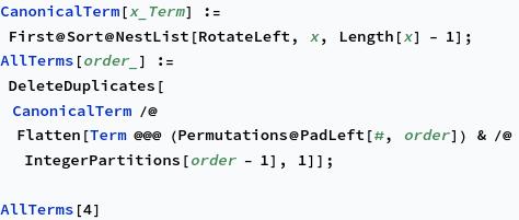
Let’s test this out! First, some quick functions to generate all the terms:

Then we need a way of converting the terms into the summations they represent:
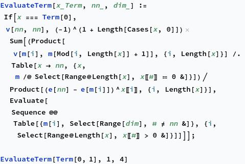

We’d like to do a numerical check, so we need a way of numerically evaluating these expressions:
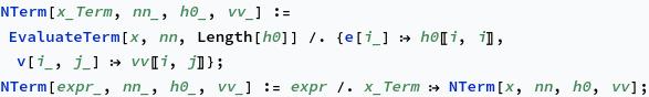
Great. Now we can define $H_0$ and $V$ and compute an expansion of an eigenvalue in two different ways:
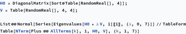

The coefficients of the corrections match up exactly!
Catalan Enumeration
It’s not hard at this point to see that $E_n^{(k)}$ seems to have $C_k$ terms:

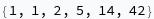
We can prove this easily now that we’ve represented terms as simple combinatorial species, namely cyclic arrangements of $k$ numbers summing to $k-1$. First, ignore the cyclic symmetry; then we can think of $k-1$ beads and $k-1$ bars separating them. For instance, [0 1 0 0 3] would be

There are then $\binom{2k-2}{k-1}$ ways of choosing where the beads go. Then we can account for the rotational symmetry simply by dividing by $k-1$ for all the ways we can rotate the arrangement (you should check that the only way to rotate one of these arrangements into itself is by a full rotation). Thus, the number of terms in perturbation theory at order $k$ is
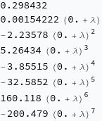
\[n_k = \frac{1}{k-1}\binom{2k-2}{k-1} = C_{k-1}.\]This is very neat. Better yet, we can actually put this to use. Let’s consider a very simple case of perturbation theory, ith
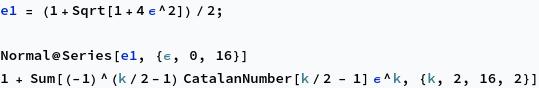
\[H_0 = \begin{pmatrix} 0 & 0 \\ 0 & 1 \end{pmatrix}, \qquad V = \begin{pmatrix} 0 & 1 \\ 1 & 0 \end{pmatrix}.\]We can easily diagonalize $H_0 + \epsilon V$ exactly, giving
\[E_0 = \frac{1}{2}\left(1 - \sqrt{1+4\epsilon^2}\right), \qquad E_1 = \frac{1}{2}\left(1 + \sqrt{1+4\epsilon^2}\right).\]Because there are only two states, the sums over $m\neq n$ appearing in perturbation theory all reduce to a single term. Let’s look at $E_1$, so that all the factors of $E_1-E_0$ in the denominator are just 1. If we have a term with two consecutive zeroes or two consecutive non-zeroes, then we have a factor of $\braket{0|V|0}$ or $\braket{1|V|1}$, both of which are zero, so we have to interlace zeroes and non-zeroes. This is only possible for even $k$, immediately showing that $E_1$ is an even function of $\epsilon$. At even $k$, we only need to consider the interlaced terms, which correspond to cycles of $k/2$ positive integers adding to $k-1$. These will all come with a factor of $(-1)^{k/2-1}$ from the number of zeroes. To count them, we repeat the argument above, which gives $\frac{2}{k}\binom{k-2}{k/2-1} = C_{k/2-1}$. Thus, by explicitly computing every term in perturbation theory (!), we find
\[E_1 = 1 + \sum_{k\text{ even}} (-1)^{k/2} C_{k/2-1}\epsilon^k.\]Comparing our exact expression for $E_1$ above with the generating function for the Catalan numbers, we find that these agree. Indeed: