Tropical Geometry of ReLU Neural Nets
Tropical Geometry of Deep Neural Networks (Zhang, Naitzat, and Lim)
 Download the notebook
A rectified linear unit (ReLU) is a neuron with activation function
\[\sigma(x) = \begin{cases} x & \text{if }x>0 \\ 0 & \text{otherwise}\end{cases}.\]A ReLU neural network is formed entirely from such units.
ReLU networks are interesting from a mathematical standpoint because the nonlinearity of $\sigma$ is in some sense as small as possible: for any $x\neq 0$, there is an open neighborhood of $x$ on which $\sigma$ is linear. Only at $x = 0$ does $\sigma$ add nonlinear effects to the network. This makes it simpler to understand these networks from an analytic standpoint, as we will see.
It is tempting to think that ReLU networks might be less powerful than networks employing a sigmoid or hyperbolic tangent activation function, because they include “less” nonlinearity per neuron. However, ReLU networks can perform quite well even on real, high-dimensional tasks. For instance, we can use a ReLU network to classify handwritten digits in the MNIST data set.
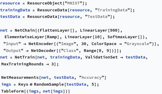

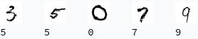
This is pretty impressive work for a piecewise linear function. (There is also a softmax layer, but we can think of this as a method for converting continuous output into classification output; none of the essential “intelligent” work happens in the softmax layer).
Given that the piecewise nonlinearity in ReLU networks can give rise to interesting and useful behavior, it is useful to try to understand and parametrize the origin of complexity in ReLU neural nets. In particular, we can use ReLU networks as a toy model to study a broader question: what is the source of the implicit regularization which allows neural networks to generalize surprisingly well to data not seen during training?
These are the goals of the paper by Zhang et al. linked in the title. They expose the relationship between ReLU neural networks and rational functions over the tropical semiring, which are well-studied in the context of algebraic geometry. Below we will give an overview of tropical algebra and the rudiments of tropical geometry, and then give a proof that the set of functions which can be expressed as ReLU neural networks (with mild integrality assumptions) is exactly the set of tropical rational functions. We then discuss some of the results bounding the complexity of ReLU networks by using this duality with tropical functions.
Tropical Geometry
Tropical geometry is the study of polynomial functions over the tropical semiring. The tropical semiring consists of $(\mathbb{R}, -\infty)$ together with the operations \(\begin{align} x\oplus y &= \max(x, y), \\ x\otimes y &= x + y. \end{align}\) To check that this forms a semiring, we must in particular check that distributivity holds. Indeed, \[x\otimes (y\oplus z) = x + \max(y, z) = \max(x + y, x + z) = x\otimes y + x \otimes z.\] In addition, we need an additive identity and a multiplicative identity. These are easily found to be $-\infty$ and 0 respectively.
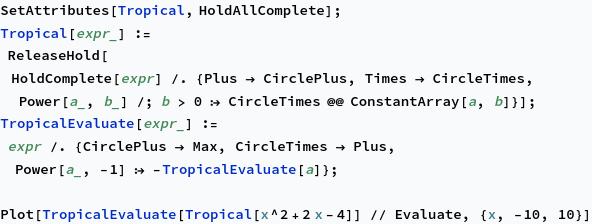
Tropical polynomials are piecewise linear functions. For instance, consider $(x\otimes x) \oplus (2\otimes x) \oplus -4$. Using the definitions of $\oplus$ and $\otimes$, we find that this is $\max(2x, x + 2, -4)$, and clearly this is piecewise linear with discontinuities at $x = -6$ and $x = 2$. Doing tropical arithmetic is a simple matter of replacing addition with maximization and multiplication with addition:
It’s clear that any tropical polynomial is a piecewise linear function. However, it’s also clear that not every piecewise linear function is a tropical polynomial. A function $f:\mathbb{R}\to\mathbb{R}$ is a tropical polynomial if and only if it is piecewise linear, convex, and $f’(x)\in \mathbb{N}$ wherever $f’(x)$ is defined. This can be proved easily by explicitly constructing a tropical polynomial to represent a function of this kind.
The requirement that $f’(x)\in \mathbb{N}$ is not especially restrictive. If $f$ has arbitrary real slopes, we can approximate them by rational numbers and multiply $f$ by some constant to get a function with integer slopes. However, convexity is a major restriction. For classification purposes, we care about sets of the form ${x\mid f(x)\ge a}$, and convexity implies that these are all of the form $(c,\infty)$, which is not useful.
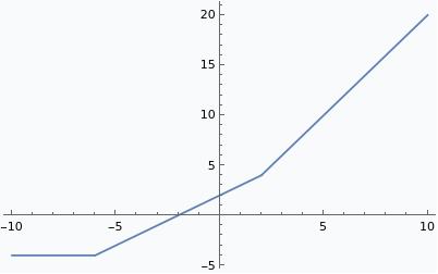
We can remove the convexity restriction by allowing tropical rational functions; that is, quotients of tropical polynomials. Division in tropical arithmetic corresponds to subtraction in ordinary arithmetic, so quotients of tropical polynomials correspond to differences of piecewise-linear, convex, integer-sloped functions. A straightforward but technical argument shows that any piecewise-linear function with integer slopes can be represented in this way. For instance, a triangle wave:

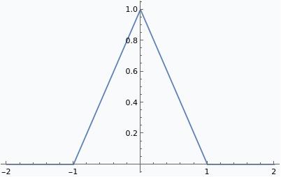
The same is true for functions $f:\mathbb{R}^d\to \mathbb{R}$: $f$ is a tropical rational function if and only if $f$ is piecewise linear with gradients $\nabla f \in \mathbb{Z}^d$. For instance, consider the tropical polynomial $x_1^2 + 2x_1x_2 + x_2^2 + 2x_1 + 2x_2 + 2$. If we plot this, we find

The white lines show where Mathematica is unsure how to plot the function because two or more monomials have the same value. This plotting artifact actually corresponds to the key object in tropical geometry, the tropical hypersurface, which is the set of points at which the value of $f$ is attained at two or more of the monomials in $f$.
The tropical hypersurface is related to another object associated with a tropical polynomial (or any polynomial), the Newton polygon. If $f = \sum c_i x^{\alpha_i}$, where $\alpha_i \in \mathbb{N}^d$ are tuples giving the exponents of each variable $x_j$, then the Newton polygon is the convex hull of all the $\alpha_i$. That is,
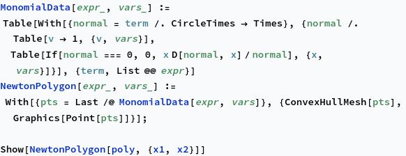

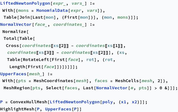
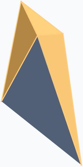
We can form a subdivision of the Newton polygon by taking the coefficients of the monomials into account. The convex hull of the points $(\alpha_i, c_i)\in \mathbb{N}^d\times \mathbb{R}$ is denoted $\mathcal{P}(f)$, and if we project the upper faces of $\mathcal{P}(f)$ down onto the Newton polygon, we get a subdivision. First, let’s compute $\mathcal{P}(f)$ and its upper faces:
Projecting these down, we get a subdivision of the Newton polygon.
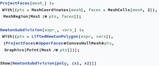
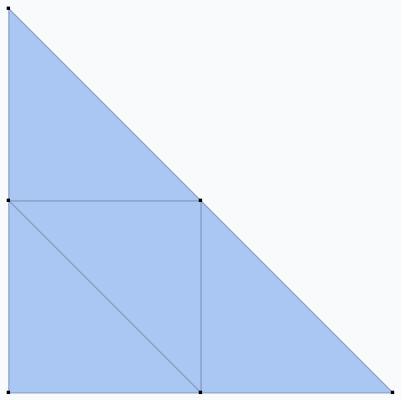
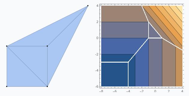
If we think of this subdivision as a graph, then it turns out to be dual to the tropical hypersurface, in the sense that each vertex of $\mathcal{P}(f)$ corresponds to a “cell” in the hypersurface of $f$, and two vertices are joined by a line in the subdivision if the corresponding two cells are adjacent. For instance, this implies that in order to get a closed loop in the tropical hypersurface, we need to have a vertex in the subdivision which is internal, as the following example shows.

This means that the number of vertices of $\mathcal{P}(f)$ is an upper bound on the number of linear regions of $f$, which we call $\mathcal{N}(f)$. Such a relationship between the geometry of $\mathcal{P}(f)$ and the $\mathcal{N}(f)$ is useful, because the latter is a measure of the complexity of $f$.
ReLU Networks
We’ve already discussed the idea that all piecewise linear functions are tropical rational functions. Now we’ll see how all piecewise linear functions are also ReLU neural networks, again focusing on the one dimensional case $f:\mathbb{R}\to\mathbb{R}$.
As an example, the triangle wave we computed earlier as a tropical rational function can also be represented by a composition of $\sigma$ (which Mathematica calls Ramp) and linear functions:


It’s easy to see how such a representation can be turned into a tropical rational function. We replace $\sigma(x)$ with $x\oplus 0$, and $ax+b$ with $bx^a$. Applying this to the function above, we find \[\sigma(\sigma(x+1) - 2\sigma(x)) \mapsto \frac{1\otimes x\oplus 0}{x^2\oplus 0} \oplus 0 = \frac{x^2 \oplus 1\otimes x \oplus 0}{x^2 \oplus 0},\] which is the tropical rational function we used above to represent this function.
To represent an arbitrary piecewise linear function as a ReLU network, we simply enumerate its discontinuities $x_i$ and their slope changes $\Delta m_i$, with $i=1,\ldots,n$. Let $m_0 x + b_0$ be the linear function which matches $f$ as $x\to -\infty$. Then we have \[f(x) = m_0 x + b + \sum_{i=1}^n \Delta m_i \sigma(x-x_i).\] For instance, the triangle wave can be written as \[\sigma(x+1) - 2\sigma(x) + \sigma(x-1),\] which gives the tropical rational function \[\frac{(1\otimes x \oplus 0)\otimes(-1 \otimes x \oplus 0)}{x^2+0} = \frac{x^2 \oplus 1\otimes x \oplus 0}{x^2\oplus 0},\] as we should expect.
The general fact, given as Theorem 5.4 of Zhang, Naitsat, and Lim, is that
Choosing $\sigma$ in this slightly more general way allows for the identity function as well, by setting $t^{(l)} = -\infty$; in the following we will continue to let $\sigma(x) = \max(x, 0)$ for simplicity.
This equivalence in itself is interesting, but not hard to anticipate: both ReLU networks (with integer weights) and tropical rational functions represent piecewise linear functions, so naturally they can represent each other. More interesting is that we can explicitly construct a tropical rational function from a ReLU network, as in the one-dimensional examples above.
It is relatively easy to generalize our method of converting ReLU networks to tropical rational functions, and in doing so we will obtain tropical algebraic formulas which will be useful in the following. Let the values of the nodes of the $i$th layer of the network be given by $n^{(i)}_j(x) = f^{(i)}_j(x)-g^{(i)}_j(x)$, where $f$ and $g$ are tropical polynomials on the input variables $x$ (and their difference is the tropical quotient). We need to compute
$$n^{(i+1)}_k(x) = \sigma\left(a_{kj} n^{(i)}_j(x) + b_k\right)$$
as a tropical rational function. Let $a_{kj} = a^+_{kj} - a^-_{kj}$, where $a^+_{kj}$ and $a^-_{kj}$ are both positive. Then it is simple to show using the rules of tropical arithmetic that
$$ \begin{align} \begin{split} n^{(i+1)}_k(x) =\, &\left(\left(\prod \left(f^{(i)}_j\right)^{a^+_{kj}}\right)\otimes\left(\prod \left(g^{(i)}_j\right)^{a^-_{kj}}\right)\otimes b_k\right) \\ -&\left(\left(\prod \left(f^{(i)}_j\right)^{a^-_{kj}}\right)\otimes\left(\prod \left(g^{(i)}_j\right)^{a^+_{kj}}\right)\right) \end{split} \end{align} $$
We can also give a reverse construction of a ReLU network from a tropical rational function. We do this by induction. To compute a tropical sum $p\oplus q$, we may use \[\max(p, q) = \sigma(p-q) + \sigma(q) - \sigma(-q).\] Thus, if $f$ and $g$ are tropical polynomials, represented by neural networks of depths $d_p$ and $d_q$, then $f\oplus g$ can be represented with a network of no more than $\max(d_p, d_q) + 1$ layers, simply by adding a layer to compute $\max(f, g)$ with the formula above. It follows that we can take any tropical polynomial $f$, form 1-layer networks to compute each of its monomials, and then join these together in pairs until we have a single network to compute $f$. This shows that the network needs at most $\lceil\log_2 r_f\rceil + 1$ layers, where $r_f$ is the number of monomials in $f$. Similarly, to compute a tropical rational function $\frac{f}{g}$, we need at most $\lceil\log_2\max{r_f,r_g}\rceil + 2$ layers.
Geometric Complexity
The main result of the paper is Theorem 6.3 concerning the number of linear regions of a ReLU neural network, which as discussed above is taken to be a measure of the complexity of the network. Using the duality between the tropical hypersurface, which determines the number of linear regions, and the Newton polygon, which is more directly accessible from an algebraic standpoint, the authors deduce a bound on the number of linear regions in terms of the depth and width of the network. The key finding is that the number of linear regions is bounded polynomially in the width, but exponentially in the depth. The exact theorem is as follows.
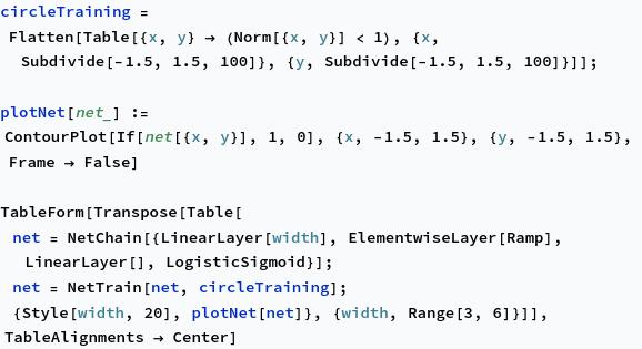
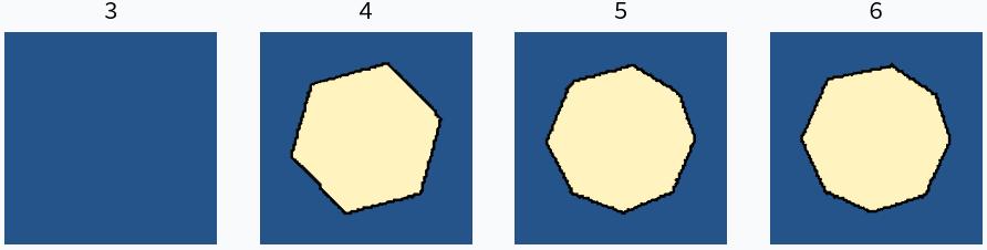
We can see the polynomial growth in complexity as a function of network width by looking at a toy example of training a network to learn a circular boundary. A ReLU network cannot learn a circular boundary exactly, and so it will be forced to approximate it by a polygon. The number of edges of the polygon is bounded by the number of linear regions in the network.
Below we see that a network with a single ReLU layer of width $n$ can learn a decision boundary which is a $2n$-gon. This is consistent with the claim that network complexity grows only polynomially in the width.